If any of you have tried to use my previous instructions on how to use manim you’ll find they no longer work with the latest editions. Updating these instructions is quite an undertaking and given my teaching load, isn’t something I can keep doing. On top of that, a number of people have taken over this task and exceeded what I set out to do with my posts originally.
If you are just getting started using manim, here are my recommendations to you:
Start out installing the Community Edition. It is more stable than the version that Grant updates, and much better documented. Follow the installation instructions on this site.
Take a look at the documentation for using manim. This wasn’t around back is 2018 but has grown to be very helpful. The documentation includes links to some tutorials.
Join the Discord server for the Community Edition of manim. If you have questions or installation issues, you can find someone who will help on Discord.
Check out the r/manim community on Reddit. There are some good examples of what people are doing with manim.
Trying to figure out manim when there wasn’t any documentation back in 2018 was a lot of fun and I’d like to think I helped kickstart the wonderful community that has grown up around manim. I’m moving on to create manim-based videos for some of my classes and it’s been long enough since I’ve used manim that I’ll be relying on tutorials created by others.
I got a new Mac from work and I didn’t have manim installed. However, when I followed my own instructions I ran into issues. I don’t know if others will have similar problems but I thought I’d document my solution just in case.
First you need a directory to clone the manim files into. I typically include the month and year in my directory title since some of my files only compile in specific versions of manim. You can clone the repository with: git clone https://github.com/3b1b/manim.git
Previously the following had worked for me: conda create --name manim --file requirements.txt but I run into a number of errors here.
Next I tried following the directions on the manim site (crazy, I know) so I tried the following:
Create a clean virtual environment: conda create --name manim_env
Unfortunately pip is not installed in a clean conda environment so I need to try: conda install pip
I tried pip install manimlib again but ran into an issue with pkg-config not being present so I had to add in:
conda install pkg-config
Now I can install manim: pip install manimlib
Just to make sure everything installed correctly I try compiling a project: python3 -m manim example_scenes.py SquareToCircle -pl
TLDR: Summary of installation (assuming conda is already installed). From within the directory where you want manim installed you can do the following:
Update as of May 2021: These instructions are now hopelessly out of date. See this post for tips on where to go for tutorial help using manim.
I previously wrote a series of blog posts detailing how to use manim, the mathematical animation package created by Grant Sanderson of 3Blue1Brown. Since I’ve written those posts there have been many changes to manim, including switching to Python 3.7. I will go through and update my information for the version of manim as of December, 2018. Much of the information will be a repeat of earlier posts in situations where there have been no changes to the manim code. The primary changes from my previous series of posts are related to changes to manim, primarily in dealing with 3D scenes. Note that future versions may break some of these commands, but hunting down the problems is the best way to learn the inner workings of manim.
1.0 Installing manim
Brian Howell has put together a really nice post on how to install the necessary components of manim at http://bhowell4.com/manic-install-tutorial-for-mac/. One of the most useful tips for making sure everything works is to use virtual environments. If you have trouble getting manim working I suggest asking for help on the github page for manim since that has an active group of users who can typically help out.
The Readme docs on github also have instructions on installing manim.
To make sure you installation is working you can run the example file that comes with manim. Type python -m manim example_scenes.py -pl. If this produces errors you should check out the Issues tab on the github site since frequently someone else has had the same issue.
2.0 Creating Your First Scene
You can copy and paste the code below into a new text file and save it as manim_tutorial_P37.py in the top-level manim directory or you can download all of the tutorials at https://github.com/zimmermant/manim_tutorial/blob/master/manim_tutorial_P37.py. The .py extension tells your operating system that this is a Python file.
Open up a command line window and go to the top-level manim directory, and type python -m manim pymanim_tutorial_P37.py Shapes -pl
We are calling the Python interpreter with the python command. If you have multiple versions of Python installed you may need to call python3 rather than just python (I use Anaconda virtual environments to keep all manim-related Python code in one handy place).
The first argument passed to Python, manim is running manim.py in the main manim directory (we’ll ignore the -m switch, which you should include). It looks like you can live-stream the output to Twitch but I’m not using that feature so I’ll focus on extract_scene.py, which is called from manim.py and which is the code that runs your script and creates a video file. The second argument, manim_tutorial_P37.py is the name of the file (i.e. the module) where your script is stored. The third argument, Shapes is the name of the class (i.e. the scene name) defined within your file that gives instructions on how to construct a scene. The last arguments, -pl tell the extract_scene script to preview the animation by playing it once it is done and to render the animation in low quality, which speeds up the time to create the animation. Typing python -m manim --help will pull up a list of the different arguments you can use when calling python -m manim.
from big_ol_pile_of_manim_imports import *

class Shapes(Scene):
    #A few simple shapes
    def construct(self):
        circle = Circle()
        square = Square()
        line=Line(np.array([3,0,0]),np.array([5,0,0]))
        triangle=Polygon(np.array([0,0,0]),np.array([1,1,0]),np.array([1,-1,0]))

        self.add(line)
        self.play(ShowCreation(circle))
        self.play(FadeOut(circle))
        self.play(GrowFromCenter(square))
        self.play(Transform(square,triangle))
If everything works you should see the following messages (or something similar) in your terminal:
The first line in the command terminal tells you where the video file is being saved. The next several lines list the name of the animation commands that you called, along with some information about how long it took for each animation and other info I don’t understand. The last line just lets you know how many animations were called in your script.
The video should look like this:
All of the various manim modules are contained in big_ol_pile_of_manim_imports.py so importing this gives you all of the basic features of manim. This doesn’t include every single module from manim but it contains the core modules. You can look at the modules included here. It is worth your time to dive into some of the modules to see how things are put together. I’ve learned a surprising amount of Python by trying to figure out how things work. Incidentally I find using the search box at https://github.com/3b1b/manim very helpful for finding different classes and figuring out what arguments they take and how they work. Documentation is also being put together for manim here, although it is still a work in progress.
2.1 Scenes and Animation
The Scene is the script that tells manim how to place and animate your objects on the screen. I read that each 3blue1brown video is created as individual scenes which are stitched together using video editing software. You must define each scene as a separate class that is a subclass of Scene. This class must have a construct() method, along with any other code required for creating objects, adding them to the screen, and animating them. The construct() method is essentially the main method in the class that gets called when run through extract_scene.py (which is called by the manim.py script). It is similar to __init__; it is the method that is automatically called when you create an instance of any subclass of Scene. Within this method you should define all of your objects, any code needed to control the objects, and code to place the objects onscreen and animate them.
For this first scene we’ve created a circle, a square, a line, and a triangle. Note that the coordinates are specified using numpy arrays np.array(). You can pass a 3-tuple like (3,0,0), which works sometimes, but some of the transformation methods expect the coordinates to be a numpy array.
One of the more important methods from the Scene() class is the play() method. play() is what processes the various animations you ask manim to perform. My favorite animation is Transform, which does a spectacular job of morphing one math object (a mobject) into another. This scene shows a square changing into a triangle, but you can use the transform to morph any two objects together. To have objects appear on the screen without any animation you can use add() to place them. The line has been added and shows up in the very first frame, while the other objects either fade in or grow. The naming of the transformations is pretty straight forward so it’s usually obvious what each one does.
Things to try – Change the order of the add() and play() commands. How does changing the order affect when they appear on the screen. – Try using the Transform() method on other shapes. – Check out the shapes defined in geometry.py which is located in the /manim/manimlib/mobject/ folder.
3.0 More Shapes
You can create almost any geometric shape using manim. You can create circles, squares, rectangles, ellipses, lines, and arrows. Let’s take a look at how to draw some of those shapes.
You can download the completed code here: manim_tutorial_P37.py. After downloading the tutorial file to your top level manim directory you can type the following into the command line to run this scene: python -m manim manim_tutorial_P37.py MoreShapes -pl.
You’ll notice we have a few new shapes and we are using a couple of new commands. Previously we saw the Circle, Square, Line, and Polygon classes. Now we’ve added Rectangle, Ellipse, Annulus, Arrow, and CurvedArrow. All shapes, with the exception of lines and arrows, are created at the origin (center of the screen, which is (0,0,0)). For the lines and arrows you need to specify the location of the two ends.
For starters, we’ve specified a color for the square using the keyword argument color=. Most of the shapes are subclasses of VMobject, which stands for a vectorized math object. VMobject is itself a subclass of the math object class Mobject. The best way to determine the keyword arguments you can pass to the classes are to take a look at the allowed arguments for the VMobject and Mobject class. Some possible keywords include radius, height, width, color, fill_color, and fill_opacity. For the Annulus class we have inner_radius and outer_radius for keyword arguments.
A list of the named colors can be found in the COLOR_MAP dictionary located in the constant.py file which is located in the /manim/manimlib/ directory. The named colors are keys to the COLOR_MAP dictionary which yield the hex color code. You can create your own colors using a hex color code picker and adding entries to COLOR_MAP.
3.1 Direction Vectors
The constants.py file contains other useful defintions, such as direction vectors that can be used to place objects in the scene. For example, UP is a numpy array (0,1,0), which corresponds to 1 unit of distance. To honor the naming convention used in manim I’ve decided to call the units of distance the MUnit or math unit (this is my own term, not a manim term). Thus the default screen height is 8 MUnits (as defined in constants.py). The default screen width is 14.2 MUnits.
If we are thinking in terms of x-, y-, and z-coordinates, UP is a vector pointing along the positive y-axis. RIGHT is the array (1,0,0) or a vector pointing along the positive x-axis. The other direction vectors are LEFT, DOWN, IN, and OUT. Each vector has a length of 1 MUnit. After creating an instance of an object you can use the .move_to() method to move the object to a specific location on the screen. Notice that the direction vectors can be added together (such as UP+LEFT) or multiplied by a scalar to scale it up (like 2*RIGHT). In other words, the direction vectors act like you would expect mathematical vectors to behave. If you want to specify your own vectors, they will need to be numpy arrays with three components. The center edge of each screen side is also defined by vectors TOP, BOTTOM, LEFT_SIDE, and RIGHT_SIDE.
The overall scale of the vectors (the relationship between pixels and MUnits) is set by the FRAME_HEIGHT variable defined in constants.py. The default value for this is 8. This means you would have to move an object 8*UP to go from the bottom of the screen to the top of the screen. At this time I don’t see a way to change it other than by changing it in constants.py.
Mobjects can also be located relative to another object using the next_to() method. The command arrow.next_to(circle,DOWN+LEFT) places the arrow one MUnit down and one to the left of the circle. The rectangle is then located one MUnit down and one left of the arrow.
The Circle class has a surround() method that allows you to create a circle that completely encloses another mobject. The size of the circle will be determined by the largest dimension of the mobject surrounded.
3.2 Making Simple Animations
As previously mentioned, the .add() method places a mobject on screen at the start of the scene. The .play() method can be used animate things in your scene.
The names of the animations, such as FadeIn or GrowFromCenter, are pretty self-explanatory. What you should notice is that animations play sequentially in the order listed and that if you want multiple animations to occur simultaneously, you should include all those animations in the argument of a single .play() command separated by commas. I’ll show you how to use lists of animations to play multiple animations at the same time later.
Things to try: – Use the Polygon class to create other shapes – Try placing multiple objects on the screen at various locations using next_to() and move_to() – Use surround() to draw a circle around objects on the screen – Take a look at the different types of transformations available in /manim/manimlib/animation/transforms.py
4.0 Creating Text
There is a special subclass of Mobject called a TextMobject (a textmath object) that can be found in tex_mobject.py. Type python -m manim manim_tutorial_P37.py AddingText -pl at the command line. Note that the text looks really fuzzy because we are rending the animations at low quality to speed things up. With a small file like this you could render it at full resolution without taking too much time. To do this, replace -pl with -p (leaving off the low resolution tag).
class AddingText(Scene):
    #Adding text on the screen
    def construct(self):
        my_first_text=TextMobject("Writing with manim is fun")
        second_line=TextMobject("and easy to do!")
        second_line.next_to(my_first_text,DOWN)
        third_line=TextMobject("for me and you!")
        third_line.next_to(my_first_text,DOWN)

        self.add(my_first_text, second_line)
        self.wait(2)
        self.play(Transform(second_line,third_line))
        self.wait(2)
        second_line.shift(3*DOWN)
        self.play(ApplyMethod(my_first_text.shift,3*UP))
To create a textmobject you must pass it a valid string as an argument. Text rendering is based on Latex so you can use many Latex typesetting features; I’ll get into that later. As a subclass of Mobjects, any method such as move_to(), shift(), and next_to() can be used with textmobjects.
The wait() method will prevent the next command for the scene from being executed for the desired number of seconds. The default time is 1 second so calling self.wait() will wait 1 second before executing the next command in your script.
You should notice that, during the animation, the second line jumps down while the top line gently glides up. This has to do with the fact that we applied the shift() method to the second line but we created an animation of the shift to the first line. When animating a mobject() method (like shift(), next_to() or move_to()), the ApplyMethod() animation is needed inside of a play() command. The shift() method by itself moves the mobject while using ApplyMethod() will animate the motion between the starting and ending points. Notice the arguments of ApplyMethod() is a pointer to the method (in this case my_first_text.shift without any parentheses) followed by a comma and then the what you would normally include as the argument to the shift() method. In other words, ApplyMethod(my_first_text.shift,3*UP) will create an animation of shifting my_first_text three MUnits up.
4.1 Changing Text
Try running the AddMoreText scene.
class AddingMoreText(Scene):
    #Playing around with text properties
    def construct(self):
        quote = TextMobject("Imagination is more important than knowledge")
        quote.set_color(RED)
        quote.to_edge(UP)
        quote2 = TextMobject("A person who never made a mistake never tried anything new")
        quote2.set_color(YELLOW)
        author=TextMobject("-Albert Einstein")
        author.scale(0.75)
        author.next_to(quote.get_corner(DOWN+RIGHT),DOWN)

        self.add(quote)
        self.add(author)
        self.wait(2)
        self.play(Transform(quote,quote2),
          ApplyMethod(author.move_to,quote2.get_corner(DOWN+RIGHT)+DOWN+2*LEFT))

        self.play(ApplyMethod(author.scale,1.5))
        author.match_color(quote2)
        self.play(FadeOut(quote))
Here we see how to change the color of text using set_color(). This uses the same colors discussed in relation to drawing geometric shapes, many of which are defined in the COLOR_MAP dictionary in constants.py. In addition to setting the color, you can also match the color to another object. In the second to last line of code above we use match_color() to change the color of the author to match quote2.
You can change the size of text using scale(). This method scales the mobject up by the numerical factor given. Thus scale(2) will double the size of a mobject while scale(0.3) will shrink the mobject down to 30% of its current size.
You can align mobjects with the center of the edge of the screen by telling to_edge() whether you want the object to be UP, DOWN, LEFT, or RIGHT. You can also use to_corner(), in which case you need to combine two directions such as UP+LEFT to indicate the corner.
Each mobject has a bounding box that indicates the outermost edges of the mobject and you can get the coordinates of the corners of this bounding box using get_corner() and specifying a direction. Thus get_corner(DOWN+LEFT) will return the location of the lower left corner of a mobject. In our example we find the lower right corner of quote and place the author one unit down from that point. Later we move the author down and slightly left of quote2.
An important thing to note is that the Transform() animation still leaves the mobject quote on the screen but has just changed its display text and properties to be those of quote2. This is why FadeOut() refers to quote and not quote2. However, the corner of quote is where it was originally, which is why we have to find the corner of quote2 to move author to the correct location. Keep in mind that when you use Tranform, properties of the mobects involved might not be what you think they are so user beware.
Another useful piece of information is that the scale() method changes the size of the objects as it currently is. In other words, using scale(.5) followed by scale(.25) results in an object that is times the original size and not as you might think.
Things to try: – Compare using .shift(), next_to(), and move_to() to applying them with the ApplyMethod() method – Try using the to_corner() method – Check out COLOR_MAP in the constants.py file and change the color of the text
4.2 Rotating and Highlighting Text
The following code will demonstrate how to rotate text and give it some pizzazz. Go ahead and run python -m manim manim_tutorial_P37.py RotateAndHighlight -p
class RotateAndHighlight(Scene):
    #Rotation of text and highlighting with surrounding geometries
    def construct(self):
        square=Square(side_length=5,fill_color=YELLOW, fill_opacity=1)
        label=TextMobject("Text at an angle")
        label.bg=BackgroundRectangle(label,fill_opacity=1)
        label_group=VGroup(label.bg,label)  #Order matters
        label_group.rotate(TAU/8)
        label2=TextMobject("Boxed text",color=BLACK)
        label2.bg=SurroundingRectangle(label2,color=BLUE,fill_color=RED, fill_opacity=.5)
        label2_group=VGroup(label2,label2.bg)
        label2_group.next_to(label_group,DOWN)
        label3=TextMobject("Rainbow")
        label3.scale(2)
        label3.set_color_by_gradient(RED, ORANGE, YELLOW, GREEN, BLUE, PURPLE)
        label3.to_edge(DOWN)

        self.add(square)
        self.play(FadeIn(label_group))
        self.play(FadeIn(label2_group))
        self.play(FadeIn(label3))
We’ve added a square in the background to show what BackgroundRectangle does. Note that the opacity of the fill color defaults to zero so if you don’t define the fill_opacity you only see the edges of the square. To create a background rectangle you need to specify the textmobject to apply this method to, as well as the opacity. You can’t change the color background to anything but black.
The VGroup class allows you to combine multiple mobjects into a single vectorized math object. This allows you to apply any VMobject methods to the all elements of the group. You are still able change properties of the original mobjects after they are added to a group. In other words, the original mobjects are not destroyed, the vmobject is just a higher level grouping of the mobjects. By grouping the text and the background rectangle we can then use rotate() to change the orientation of both objects together. Note that TAU is equal to (see the Tau Manifesto, which makes some interesting points).
The next_to() method can be thought of as a shift relative to some other object so label2_group.next_to(label_group,DOWN) places label2_group shifted down one unit from label1_group (remember that the unit of distance is set by the FRAME_HEIGHT variable in constants.py and the default screen height is 8 units).
You can create a a color gradient using set_color_by_gradient(). Pass the method any number of colors, separated by commas.
Things to play with – Try changing the fill opacity for both the square and the background rectangle – Try rotating the background rectangle separately from the the text – Change the color of label2 to see how it affects the readability of the text – Change the colors of “Rainbow” – Place the “Rainbow” text on a different edge of the screen.
5.0 Mathematical Equations
A math animation package wouldn’t be much use if you couldn’t include nice looking equations. The best way I know of to typeset equations is using LaTeX () , which manim makes use of. If you’d like to learn more about typesetting with LaTeX I’d recommend the tutorials at ShareLaTeX for a basic intro, but you don’t need to know much about LaTeX to use manim. You can find a list of commonly used symbols here, which is about all you need to know for manim.
Use manim to run the following scene from the tutorial file to see the following scene:
class BasicEquations(Scene):
    #A short script showing how to use Latex commands
    def construct(self):
        eq1=TextMobject("$\\vec{X}_0 \\cdot \\vec{Y}_1 = 3$")
        eq1.shift(2*UP)
        eq2=TexMobject(r"\vec{F}_{net} = \sum_i \vec{F}_i")
        eq2.shift(2*DOWN)

        self.play(Write(eq1))
        self.play(Write(eq2))
In LaTeX you normally enclose an equation with dollar signs $$ to denote an equation and that works here as well. The main difference is that, due to how manim parses the text, an extra backslash must be included in front of all LaTeX commands. For instance Greek letters can be created in LaTeX by typing out the name of the letter preceded by a backslash; lower case alpha would be $\alpha$, the angle theta would be $\theta$. In manim, however, a double backslash is needed so would be $\\alpha$ and would be written as $\\theta$.
David Bieber pointed out in a comment that you can use the raw string literal flag in front of the quote symbol, which removes the need for the double-slashes before Latex symbols. Instead of typing out eq2=TexMobject("\\vec{F}_{net} = \\sum_i \\vec{F}_i") you can put the letter r in front of the opening quotes and remove the double-slashes so eq2=TexMobject(r"\vec{F}_{net} = \sum_i \vec{F}_i"). This makes the code more readable and makes it much easier for those of us who normally type Latex. Going forward I will use the raw tag r rather than double-slashes.
You can place a vector arrow over a variable such as using \vec{A} (remember you either need to use double-slashes or use the raw string literal tag r). Whatever you place inside the brackets will show up on screen with an arrow over it. Subscripts are denoted by the underscore so would be written as $\vec{X}_0$. If the subscript consists of more than a single character you can enclose the subscript in brackets. Thus in manim would be $\vec{F}_{net}$.
It can get tedious having to always include the dollar signs so the TexMobject class (which is different than a TextMobject – notice the missing ‘t’ in the middle of the class name) assumes all strings are Latex strings. TEX () is the typesetting language that LaTeX is based on so I assume TexMobject is named for TEX. The main difference between TextMobject() and TexMobject is the text math object assumes everything is plain text unless you specify an equation with dollar signs while the Tex math object assumes everything is an equation unless you specify something is plain text using \\text{}.
When mobjects of any sort are created the default position seems to be the center of the screen. Once created you can use shift() or move_to() to change the location of the mobjects. For this example above I’ve moved the equations either two MUnits up or two MUnits down (remember that the MUnit or math unit is what I call the measure of length inside manim). Since the screen height is set to a default of 8 MUnits, a 2 MUnit shift corresponds to about a quarter of the screen height.
The Write() method, which is a sublcass of ShowCreation(), takes a TextMobject or TexMobject and animates writing the text on the screen. You can also pass a string to Write() and it will create the TextMobject for you. Write() needs to be inside of play() in order to animate it.
5.1 Coloring Equations
class ColoringEquations(Scene):
    #Grouping and coloring parts of equations
    def construct(self):
        line1=TexMobject(r"\text{The vector } \vec{F}_{net} \text{ is the net }",r"\text{force }",r"\text{on object of mass }")
        line1.set_color_by_tex("force", BLUE)
        line2=TexMobject("m", "\\text{ and acceleration }", "\\vec{a}", ".  ")
        line2.set_color_by_tex_to_color_map({
            "m": YELLOW,
            "{a}": RED
        })
        sentence=VGroup(line1,line2)
        sentence.arrange_submobjects(DOWN, buff=MED_LARGE_BUFF)
        self.play(Write(sentence))
For this example we have broken our text into blocks of plain text and equations. This allows us to color parts of the text or equations using either set_color_by_tex() or set_color_by_tex_to_color_map(). For example, the reason the first sentence is broken up into three parts is so the word force can be colored blue. As far as I can tell there isn’t an easy way in manim to make changes to part of a string. While you could use slicing of a string, I’m following the convention that Grant Sanderson uses and breaking up text into a list of strings.
The set_color_by_tex() method takes the individual string you want colors and the color as arguments. It looks like you only have to specify part of a string to match but the entire string gets colored. For instance, if we type in line1.set_color_by_tex("F",BLUE), the only place a capital F occurs is in the force variable so the first part of this line is blue. If instead we try line1.set_color_by_tex("e",BLUE), the letter e appears in several places in line1 so the entire line ends up blue. If you want to change the color of multiple elements within a list of texmobjects you can use set_color_by_tex_to_color_map() and a dictionary. The key for the dictionary should be the text we want colored (or a unique part of the string) and the value should be the desired color.
Notice that, since we are using a texmobject and not a textmobject, we have to enclose plain text in the LaTeX command \\text{}. If you don’t do this the text is assumed to be part of an equation so the font and spacing are of the text looks funny. Thus “the net force on object of mass” would look like . The equation environment doesn’t recognize spaces between words, uses a different font, and spaces the letters differently than normal text.
By grouping the two lines together with VGroup(), we can use the arrange_submobjects() method to space out the two lines. The first argument is the direction you want the objects spaced out and buff is the buffer distance between the mobjects. There are several default buffer distances defined in constants.py but you can also a single number. The smallest default buffer is SMALL_BUFF=0.1 and the largest is LARGE_BUFF=1. Although I didn’t dive into the code, I think the way the buffers work is as a multiplicative factor of one of the main directional vectors (e.g. UP, DOWN, LEFT, RIGHT) so that specifying SMALL_BUFF and LEFT would be equivalent to .
Things to try: – Create your own equations using the symbols here. – Try changing the colors of different parts of the equations – Use set_color_by_tex and match only a part of a full string to see how the entire string is changed – Write out a sentence as a single string and then use slicing to create texmobjects
6.0 Aligning Text and Using Braces
Let’s look at how to use braces to visually group equations or text together but also how to align text elements. We will first write a program to align elements of two equations but in a somewhat clunky fashion; this is not the most elegant way to accomplish this task. After looking at this first version we will rewrite the code in a more concise fashion that lines everything up even better.
class UsingBraces(Scene):
    #Using braces to group text together
    def construct(self):
        eq1A = TextMobject("4x + 3y")
        eq1B = TextMobject("=")
        eq1C = TextMobject("0")
        eq2A = TextMobject("5x -2y")
        eq2B = TextMobject("=")
        eq2C = TextMobject("3")
        eq1B.next_to(eq1A,RIGHT)
        eq1C.next_to(eq1B,RIGHT)
        eq2A.shift(DOWN)
        eq2B.shift(DOWN)
        eq2C.shift(DOWN)
        eq2A.align_to(eq1A,LEFT)
        eq2B.align_to(eq1B,LEFT)
        eq2C.align_to(eq1C,LEFT)

        eq_group=VGroup(eq1A,eq2A)
        braces=Brace(eq_group,LEFT)
        eq_text = braces.get_text("A pair of equations")

        self.add(eq1A, eq1B, eq1C)
        self.add(eq2A, eq2B, eq2C)
        self.play(GrowFromCenter(braces),Write(eq_text))
To line up parts of the equations on screen we use next_to() and align_to(). For this example we’ve broken the equation into smaller parts and then used next_to() to place the subparts of each equation next to each other and then align_to() to line up the left side of each part of the equation. You can also use UP, DOWN, and RIGHT to align different edges of the mobjects.
We’ve also added a brace to show how to visually group a set of equations. In order to use the braces we must use VGroup() to combine the equations. When we instantiate the braces the first argument is the group and the second argument is where the braces are located relative to the grouping. You can set the text next to the braces using get_text() (this is a little confusing naming because you are setting the text, not getting it). This method does not draw the text on the screen, it is only used to set the location of the text relative to the braces so you will still need to add the text to the screen.
class UsingBracesConcise(Scene):
    #A more concise block of code with all columns aligned
    def construct(self):
        eq1_text=["4","x","+","3","y","=","0"]
        eq2_text=["5","x","-","2","y","=","3"]
        eq1_mob=TexMobject(*eq1_text)
        eq2_mob=TexMobject(*eq2_text)
        eq1_mob.set_color_by_tex_to_color_map({
            "x":RED_B,
            "y":GREEN_C
            })
        eq2_mob.set_color_by_tex_to_color_map({
            "x":RED_B,
            "y":GREEN_C
            })
        for i,item in enumerate(eq2_mob):
            item.align_to(eq1_mob[i],LEFT)
        eq1=VGroup(*eq1_mob)
        eq2=VGroup(*eq2_mob)
        eq2.shift(DOWN)
        eq_group=VGroup(eq1,eq2)
        braces=Brace(eq_group,LEFT)
        eq_text = braces.get_text("A pair of equations")

        self.play(Write(eq1),Write(eq2))
        self.play(GrowFromCenter(braces),Write(eq_text))
Here is a (somewhat) more concise version of the previous code. Each equation is written out as a list with each part of the equation as a separate string. This allows more control over the vertical alignment of the parts of the two equations. Inside the for loop we use align_to() to line up the left edge of the elements in eq1 and eq2.
Notice that when creating the texmobjects that we passed the variable name of the list with an asterisk in front of it eq1_mob=TexMobject(*eq1_text). The asterisk is a Python command to unpack the list and treat the argument as a comma-separated list. Thus eq1_mob=TexMobject(*eq1_text) is identical to eq1_mob=TexMobject("4","x","+","3","y","=","0").
Things to try: – Arrange the equations on the screen – Add some shapes around your equations.
7.0 Graphing Functions
The easiest way to plot functions is to base your scene class on the GraphScene(). The scene creates a set of axes and has methods for creating graphs. One thing that confused me a little at first is that the axes belong to your scene class so you will need to use self to access the methods related to the axes. This caused me a few issues when I started out.
We will start off by looking at how to create the axes and graphs but we will come back to look at the CONFIG{} dictionary, which is used frequently in manim for initializing many of the class variables.
Under the construct method, the first line is self.setup_axes() which will create a set of axes on screen. With the exception of whether the creation is animated or not, all other variables for the axes are set using CONFIG{}, which I’ll explain in a bit. The default values for the GraphScene() (which are located in graph_scene.py) are shown below:
With our example we have changed x_min, x_max, y_min, y_max, graph_origin, axes_color, and x_labeled_num. The values assigned in our class take priority over values set by the parent class. Every value that we don’t change is automatically assigned the value defined in the parent class. The x_labeled_num property takes a list of numbers for labels along the x-axis. We’ve used range(-10,12,2) to generate a list of values from -10 to +10 in steps of 2. One issue I’ve noted with the y-axis is that setting the min values along either axis to numbers that are not integer multiples of 0.5 results in the tick marks along that axis not being symmetric about zero (e.g. try y_min = -1.2). I’m not sure what that is about but it isn’t a problem if you stick to integer multiples of 0.5 you don’t have any problems.
Once you have the axes set up you can use self.get_graph() to graph a function. The argument of get_graph() needs to be a pointer to a function, rather than a call to the function itself. In other words, since one of my functions is func_to_graph() I should use self.get_graph(func_to_graph) without any parentheses after func_to_graph.
Rather than defining separate functions for graphing we could use lambda functions. For example, if I define self.func = lambda x: np.cos(x) and then use self.get_graph(self.func) I will get the same result.
With get_graph() you do need to explicitly pass arguments rather than using CONFIG{}. The possible arguments, in addition to the function to graph, are color, x_min, and x_max. If you don’t specify a color GraphScene will cylce through BLUE, GREEN, and YELLOW for successive graphs. Since I didn’t specify a color for my second graph it was automatically assigned the first color, BLUE.
There is a handy method to draw a vertical line from the x-axis to the graph called get_vertical_line_to_graph(). I love that the method naming convention is descriptive enough that you can see what each method does at a glance. Good job, Grant! The arguments for get_vertical_line_to_graph() are the x-value where you want the line and the particular graph you want the line drawn to. Note that get_vertical_line_to_graph() is a method of the GraphScene and not the graph or axes so it is called with self.get_vertical_line_to_graph().
You can label graphs using get_graph_label() to set the text associated with the graph. This is similar to the get_text() method of the Braces() class in that it creates a texmobject at a specific location but does not draw it on the screen; you need to add or play to show the label. The arguments for get_graph_label() are the particular graph you want to add a label to and the text for the label. If you don’t specify an x-value and/or direction the label is placed at the end of the graph. The direction specifies where, relative to the x_value you want the label placed.
There are several other methods associated with the GraphScene() that are worth looking at, but I found the input_to_graph_point() to be very helpful. By specifying an x-value on the graph, this method will return the coordinate on the screen where that graph point lies. This is handy if you want to place some text or other mobject to call out a particular point on a graph.
7.1 The CONFIG{} Dictionary
Whenever a scene or mobject are created a method called digest_config() gets called. This method starts with the class you defined and looks for a dictionary called self.CONFIG and compiles a list of all entries in the dictionary. It then goes to the parent class and looks for self.CONFIG there and adds those entries. If the method comes across keys that have already been found, it ignores the values from the parent class. digest_config() keeps traveling up the hierarchy to the top parent class, with is Container(). Each entry in this dictionary is then assigned a class variable based on the key and value. Thus the dictionary entry "x_min" : -1 becomes self.x_min = -1 and so on. Each dictionary entry becomes a class variable that can be accessed by the methods within the class. Understanding all of the CONFIG{} entries for a class is crucial to getting the most out of manim. For example, GraphScene() has the following CONFIG{} entries:
class GraphScene(Scene):
CONFIG = {
    "x_min": -1,
    "x_max": 10,
    "x_axis_width": 9,
    "x_tick_frequency": 1,
    "x_leftmost_tick": None, # Change if different from x_min
    "x_labeled_nums": None,
    "x_axis_label": "$x$",
    "y_min": -1,
    "y_max": 10,
    "y_axis_height": 6,
    "y_tick_frequency": 1,
    "y_bottom_tick": None, # Change if different from y_min
    "y_labeled_nums": None,
    "y_axis_label": "$y$",
    "axes_color": GREY,
    "graph_origin": 2.5 * DOWN + 4 * LEFT,
    "exclude_zero_label": True,
    "num_graph_anchor_points": 25,
    "default_graph_colors": [BLUE, GREEN, YELLOW],
    "default_derivative_color": GREEN,
    "default_input_color": YELLOW,
    "default_riemann_start_color": BLUE,
    "default_riemann_end_color": GREEN,
    "area_opacity": 0.8,
    "num_rects": 50,
}
The parent class for GraphScene() (found in the scene.py file) has the following dictionary:
Container(), the parent to Scene as well as Mobject, has no CONFIG{} entries.
When talking about mobjects, the list of CONFIG{} entries can get a little long. I won’t go into those right now but it is worth you time to take a look at the hierarchy of some of the mobject subclasses to see what all the properties you can control are.
8.0 More Graphing
Let’s take a deeper dive into some of the graphing features in manim.
class ExampleApproximation(GraphScene):
    CONFIG = {
        "function" : lambda x : np.cos(x),
        "function_color" : BLUE,
        "taylor" : [lambda x: 1, lambda x: 1-x**2/2, lambda x: 1-x**2/math.factorial(2)+x**4/math.factorial(4), lambda x: 1-x**2/2+x**4/math.factorial(4)-x**6/math.factorial(6),
        lambda x: 1-x**2/math.factorial(2)+x**4/math.factorial(4)-x**6/math.factorial(6)+x**8/math.factorial(8), lambda x: 1-x**2/math.factorial(2)+x**4/math.factorial(4)-x**6/math.factorial(6)+x**8/math.factorial(8) - x**10/math.factorial(10)],
        "center_point" : 0,
        "approximation_color" : GREEN,
        "x_min" : -10,
        "x_max" : 10,
        "y_min" : -1,
        "y_max" : 1,
        "graph_origin" : ORIGIN ,
        "x_labeled_nums" :range(-10,12,2),

    }
    def construct(self):
        self.setup_axes(animate=True)
        func_graph = self.get_graph(
            self.function,
            self.function_color,
        )
        approx_graphs = [
            self.get_graph(
                f,
                self.approximation_color
            )
            for f in self.taylor
        ]

        term_num = [
            TexMobject("n = " + str(n),aligned_edge=TOP)
            for n in range(0,8)]
        #[t.to_edge(BOTTOM,buff=SMALL_BUFF) for t in term_num]


        #term = TexMobject("")
        #term.to_edge(BOTTOM,buff=SMALL_BUFF)
        term = VectorizedPoint(3*DOWN)

        approx_graph = VectorizedPoint(
            self.input_to_graph_point(self.center_point, func_graph)
        )

        self.play(
            ShowCreation(func_graph),
        )
        for n,graph in enumerate(approx_graphs):
            self.play(
                Transform(approx_graph, graph, run_time = 2),
                Transform(term,term_num[n])
            )
            self.wait()
I wanted to demonstrate how adding higher terms in a Taylor expansion results in better and better agreement with a function. This is similar to what shinigamiphoenix posted here.
The functions to plot are defined as lambda functions in the CONFIG{} dictionary. As previously mentioned, manim processes all elements in CONFIG{} and turns the dictionary entries into class variables with the key as the variable name. Thus "function" can be accessed within my class by calling self.function and "taylor" can be called with self.taylor. If you aren’t familiar with lambda functions, check out this post at Python Conquers the Universe.
We create a list of graphs using get_graph() and a list comprehension. You can find a nice tutorial on list comprehensions over at datacamp.com. It was only after reading this tutorial that I made the connection between list comprehensions and mathematical notation for definitions of sets (e.g. the set of positive real numbers is { R and } or the set of even numbers which is { I and }), which made list comprehensions click for me. For each item in the list self.taylor, a graph is created with color self.approximation_color. We also created a list of TexMobjects to indicate which order of terms are included from the Taylor expansion using a list comprehension.
Since we are going to do successive transformations from a list, it helps to have a blank placeholder on the screen. term and approx_graph are VectorizedPoint instances, which are mobjects that don’t display anything on screen. This way we can put the placeholders on the screen without anything appearing, and then transform those mobjects into either the graph or the TexMobjects.
The enumerate() command is a useful tool that iterates over a list and also returns the index of the item returned. Thus for n,graph in enumerate(approx_graphs) returns the index between 0 and 4 as n, and the element within the list as graph. This is used to display the corresponding item from term_num with each graph.
9.0 Vector Fields
Before diving into draw a vector field, we should set up a Cartesian axes using NumberPlane(). This gives you two axes and an underlying grid. The CONFIG{} for the NumberPlane() (found in the coordinate_systems.py file) is:
class NumberPlane(VMobject):
    CONFIG = {
        "color": BLUE_D,
        "secondary_color": BLUE_E,
        "axes_color": WHITE,
        "secondary_stroke_width": 1,
        # TODO: Allow coordinate center of NumberPlane to not be at (0, 0)
        "x_radius": None,
        "y_radius": None,
        "x_unit_size": 1,
        "y_unit_size": 1,
        "center_point": ORIGIN,
        "x_line_frequency": 1,
        "y_line_frequency": 1,
        "secondary_line_ratio": 1,
        "written_coordinate_height": 0.2,
        "propagate_style_to_family": False,
        "make_smooth_after_applying_functions": True,
    }
You can change any of these default values by passing a dictionary with new values as keyword arguments. For example, if you want to change the spacing of the grid lines you could change x_line_frequency and y_line_frequency by defining a dictionary with these variables and then passing the dictionary to NumberPlane(). If you want to see the x-axis and y-axis indicated you can use get_axis_labels() to draw an x and a y next to the appropriate axis. See the code below.
The double asterisk in front of the argument self.plane_kwargs lets the class know that this is a dictionary that needs to be unpacked.
I recommend changing the various properties to see what affect they have on the axes and grid. This is the best way to learn what things do.
9.1 A Simple Vector Field
Let’s start with a simple vector field; a constant field. We first need to define a set of vector points for each grid point, define the field at each grid point, then create the Vector() for the field at each point. Finally we combine all the Vector() instances into a VGroup to allow us to draw all vector lines with a single command.
class SimpleField(Scene):
    CONFIG = {
    "plane_kwargs" : {
        "color" : RED
        },
    }
    def construct(self):
        plane = NumberPlane(**self.plane_kwargs)
        plane.add(plane.get_axis_labels())
        self.add(plane)

        points = [x*RIGHT+y*UP
            for x in np.arange(-5,5,1)
            for y in np.arange(-5,5,1)
            ]

        vec_field = []
        for point in points:
            field = 0.5*RIGHT + 0.5*UP
            result = Vector(field).shift(point)
            vec_field.append(result)

        draw_field = VGroup(*vec_field)


        self.play(ShowCreation(draw_field))
After creating the NumberPlane() we use a list comprehension to create a list of the location of all grid points. Remember that RIGHT=np.array(1,0,0) and UP=np.array(0,1,0) so this list comprehension covers all points from (5,5,0) down to (-5,-5,0) in unit step sizes. The last number in arange() specifies the step size. Next we create an empty list vec_field to hold all of the vectors we are going to create. The for loop goes through each grid location in points and creates a vector whose length and direction are defined by field. It is inefficient to keep defining field each time through the loop but we are setting things up for later. The shift(point) command moves the vector to the grid location defined by point. These results are then appended to a list. After going through the for loop, all of the vectors are grouped together in a single VGroup called draw_field. The only reason for doing this is that you can then add draw_field using a single add or play command. You could have included self.add(result) inside each iteration of the for loop instead of showing the creation of draw_field, but using the VGroup feels cleaner.
9.2 A Variable Vector Field
For a slightly more interesting field we will look at the electric field due to a postive point charge. The electric field is:
where is the charge on the point charge, is the distance vector between the charge and the observation point, and is the magnitude of that vector. The constant out front is essentially a conversion factor. For our purposes we will set all constants equal to zero and just look at
.
class FieldWithAxes(Scene):
    CONFIG = {
    "plane_kwargs" : {
        "color" : RED_B
        },
    "point_charge_loc" : 0.5*RIGHT-1.5*UP,
    }
    def construct(self):
        plane = NumberPlane(**self.plane_kwargs)
        plane.add(plane.get_axis_labels())
        self.add(plane)

        field = VGroup(*[self.calc_field(x*RIGHT+y*UP)
            for x in np.arange(-9,9,1)
            for y in np.arange(-5,5,1)
            ])

        self.play(ShowCreation(field))


    def calc_field(self,point):
        #This calculates the field at a single point.
        x,y = point[:2]
        Rx,Ry = self.point_charge_loc[:2]
        r = math.sqrt((x-Rx)**2 + (y-Ry)**2)
        efield = (point - self.point_charge_loc)/r**3
        #efield = np.array((-y,x,0))/math.sqrt(x**2+y**2)  #Try one of these two fields
        #efield = np.array(( -2*(y%2)+1 , -2*(x%2)+1 , 0 ))/3  #Try one of these two fields
        return Vector(efield).shift(point)
The location of the point charge is set in CONFIG{}. To create the vector field we’ve condensed the previous code. We use a list comprehension and the function calc_field() as the argument of VGroup(). The calc_field() function defines the field to calculate. To make the formulas a little easier to read we unpack the x- and y-coordinates from the point vector and the self.point_charge_loc vector. The code x,y=point[:2] is equivalent to x=point[0] and y=point[1].
The fade(0.9) method sets the opacity of the lines to be one minus the fade level (so in this case the opacity is set to 0.1). This was done to make it easier to see the tiny field arrows farther from the charge location.
Things to try: – Change each of the elements in CONFIG{} for NumberPlane() to see what affect they have on the axes and grid lines. – Calculate different fields – Try efield = np.array((-y,x,0))/math.sqrt(x**2+y**2) – Try efield = np.array(( -2*(y%2)+1 , -2*(x%2)+1 , 0 ))/3 – Come up with your own equation
10.0 Field of a Moving Charge
There was a question over on Reddit about how to create the electric field of a moving charge. Since that is something I will want to do at some point I figured it would be fun to give it a try.
Before creating a changing field, I thought I’d start with moving charges around. I know I saw this in one of the videos so I can start with working code and modify it to my needs. Here is what I came up with:
class MovingCharges(Scene):
    CONFIG = {
    "plane_kwargs" : {
        "color" : RED_B
        },
    "point_charge_loc" : 0.5*RIGHT-1.5*UP,
    }
    def construct(self):
        plane = NumberPlane(**self.plane_kwargs)
        plane.add(plane.get_axis_labels())
        self.add(plane)

        field = VGroup(*[self.calc_field(x*RIGHT+y*UP)
            for x in np.arange(-9,9,1)
            for y in np.arange(-5,5,1)
            ])
        self.field=field
        source_charge = self.Positron().move_to(self.point_charge_loc)
        self.play(FadeIn(source_charge))
        self.play(ShowCreation(field))
        self.moving_charge()

    def calc_field(self,point):
        x,y = point[:2]
        Rx,Ry = self.point_charge_loc[:2]
        r = math.sqrt((x-Rx)**2 + (y-Ry)**2)
        efield = (point - self.point_charge_loc)/r**3
        return Vector(efield).shift(point)

    def moving_charge(self):
        numb_charges=4
        possible_points = [v.get_start() for v in self.field]
        points = random.sample(possible_points, numb_charges)
        particles = VGroup(*[
            self.Positron().move_to(point)
            for point in points
        ])
        for particle in particles:
            particle.velocity = np.array((0,0,0))

        self.play(FadeIn(particles))
        self.moving_particles = particles
        self.add_foreground_mobjects(self.moving_particles )
        self.always_continually_update = True
        self.wait(10)

    def field_at_point(self,point):
        x,y = point[:2]
        Rx,Ry = self.point_charge_loc[:2]
        r = math.sqrt((x-Rx)**2 + (y-Ry)**2)
        efield = (point - self.point_charge_loc)/r**3
        return efield

    def continual_update(self, *args, **kwargs):
        if hasattr(self, "moving_particles"):
            dt = self.frame_duration
            for p in self.moving_particles:
                accel = self.field_at_point(p.get_center())
                p.velocity = p.velocity + accel*dt
                p.shift(p.velocity*dt)


    class Positron(Circle):
        CONFIG = {
        "radius" : 0.2,
        "stroke_width" : 3,
        "color" : RED,
        "fill_color" : RED,
        "fill_opacity" : 0.5,
        }
        def __init__(self, **kwargs):
            Circle.__init__(self, **kwargs)
            plus = TexMobject("+")
            plus.scale(0.7)
            plus.move_to(self)
            self.add(plus)
The most important method here is continual_update(). This method updates the screen for each frame during the entire scene. This differs from the various transformations that rely on the play() method in that the transformations occur over a short time interval, usually on the order of a few seconds while the continual methods continue to run for the entire scene. If we want a particle to move across the screen we might be tempted to use something like self.play(ApplyMethod(particle1.shift,5*LEFT)) but it would be challenging to control the timing of other transformations going on at the same time. The continual_update() allows you to animate things in the background while still controlling the timing of other transformations.
Since I know I will be using charged particles in my videos I’ve written a Positron class to create positively charged particles. The positron is the positive antiparticle of the electron. Why didn’t I make it a proton? Because the proton is roughly 2000 times more massive and I want similarly sized particles for what I want to do.
We’ve reused the code from a previous post about electric fields but we’ve added methods to create the charged particles and move them around. moving_charge() is what creates positrons by randomly selecting a field point (possible_points = [v.get_start() for v in self.field] is a list of the locations of the tails of all field vectors) and then selects numb_charges points to create particles at. Note that the randomly generated charges don’t react to one another, which I find disturbing to watch because it isn’t physical.
particles is a vectorized mobject group that contains all of the moving charges with initial velocities set to zero (particle.velocity = np.array((0,0,0))). We could have simplified the code by only using one particle at a set location, but we’ll need multiple charges later on. The charges are then added to the screen (self.play(FadeIn(particles)) and assigned to a class variable that is needed in continual_update (self.moving_particles = particles). Mobjects are drawn in the order they are added to the screen but you can place certain mobjects in the foreground to insure they always remain drawn on top of other objects by using add_foreground_mobjects(). It is kind of like layers in Photoshop or similar software except each mobject is in its own layer. This has to do with the fact that manim keeps all mobjects drawn on the screen in a list and draws them in the order they are listed. There is no equivalent background mobject method, but you can send mobjects to the front or back layers with bring_to_front() and bring_to_back().
Next we tell manim to continually update things in the background (self.always_continually_update = True) and then wait ten seconds. It is important to set the wait() command because the continual update only runs as long as their are animation elements (play() commands) or wait() commands in the animation queue.
The field_at_point() method duplicates some of the earlier code but is used to return a numerical vector (a numpy 3-element array) rather than a mobject Vector, which is what calc_field() returns. It took me an embarassing amount of time to figure out why I couldn’t just use calc_field() to find the force vector.
The continual_update() method is called each frame when the scene is being composed. The first line, if hasattr(self, "moving_particles"): prevents the rest of the code running and throwing and error if you haven’t created self.moving_particles. The frame duration is either 1/15, 1/30, or 1/60 of a second, depending on whether your video is low, medium, or production quality (i.e. whether you include -l, -m, or no command line argument when extracting the scene). We run through the list of all moving particles (for p in self.moving_particles:) and then calculate the acceleration due to the electric field at the location of each particle (vect = self.field_at_point(p.get_center())). p.get_center() returns the vector location of each particle p. The velocity is updated using and then the particle is shifted over the distance .
10.1 Updating the Electric Field of a Moving Charge
Now we’ve got some experience moving things around on the screen so we can move on to calculating the field due to the particle. We will reuse much of the code from our previous program, with a few changes.
class FieldOfMovingCharge(Scene):
    CONFIG = {
    "plane_kwargs" : {
        "color" : RED_B
        },
    "point_charge_start_loc" : 5.5*LEFT-1.5*UP,
    }
    def construct(self):
        plane = NumberPlane(**self.plane_kwargs)
        #plane.main_lines.fade(.9)
        plane.add(plane.get_axis_labels())
        self.add(plane)

        field = VGroup(*[self.create_vect_field(self.point_charge_start_loc,x*RIGHT+y*UP)
            for x in np.arange(-9,9,1)
            for y in np.arange(-5,5,1)
            ])
        self.field=field
        self.source_charge = self.Positron().move_to(self.point_charge_start_loc)
        self.source_charge.velocity = np.array((1,0,0))
        self.play(FadeIn(self.source_charge))
        self.play(ShowCreation(field))
        self.moving_charge()

    def create_vect_field(self,source_charge,observation_point):
        return Vector(self.calc_field(source_charge,observation_point)).shift(observation_point)

    def calc_field(self,source_point,observation_point):
        x,y,z = observation_point
        Rx,Ry,Rz = source_point
        r = math.sqrt((x-Rx)**2 + (y-Ry)**2 + (z-Rz)**2)
        if r<0.0000001:   #Prevent divide by zero  ##Note:  This won't work - fix this
            efield = np.array((0,0,0))
        else:
            efield = (observation_point - source_point)/r**3
        return efield


    def moving_charge(self):
        numb_charges=3
        possible_points = [v.get_start() for v in self.field]
        points = random.sample(possible_points, numb_charges)
        particles = VGroup(self.source_charge, *[
            self.Positron().move_to(point)
            for point in points
        ])
        for particle in particles[1:]:
            particle.velocity = np.array((0,0,0))
        self.play(FadeIn(particles[1:]))
        self.moving_particles = particles
        self.add_foreground_mobjects(self.moving_particles )
        self.always_continually_update = True
        self.wait(10)


    def continual_update(self, *args, **kwargs):
        Scene.continual_update(self, *args, **kwargs)
        if hasattr(self, "moving_particles"):
            dt = self.frame_duration

            for v in self.field:
                field_vect=np.zeros(3)
                for p in self.moving_particles:
                    field_vect = field_vect + self.calc_field(p.get_center(), v.get_start())
                v.put_start_and_end_on(v.get_start(), field_vect+v.get_start())

            for p in self.moving_particles:
                accel = np.zeros(3)
                p.velocity = p.velocity + accel*dt
                p.shift(p.velocity*dt)


    class Positron(Circle):
        CONFIG = {
        "radius" : 0.2,
        "stroke_width" : 3,
        "color" : RED,
        "fill_color" : RED,
        "fill_opacity" : 0.5,
        }
        def __init__(self, **kwargs):
            Circle.__init__(self, **kwargs)
            plus = TexMobject("+")
            plus.scale(0.7)
            plus.move_to(self)
            self.add(plus)
One change we’ve made is to let calc_field() return a numpy vector rather than a mobject Vector. This does mean adding in create_vect_field() to create the mobjects from the numpy vectors.
Since we want our source charge to be able to move we have to add that source charge to the particles list. Thus the Vgroup we create includes that source charge plus the randomly generated charges using particles = VGroup(self.source_charge, *[self.Positron().move_to(point) for point in points]). Remember that the asterisk in front of the list lets Python know that each element in the list should be broken out and treated as a separate argument for the VGroup() class. To help make sense of this line of code we can break it out into a less elegant form:
list_of_random_charges=[]
for point in points:
    new_charge = self.Positron().move_toe(point)
    list_of_random_charges.append(new_charge)
    particles = VGroup(self.source_charge, list_of_random_charges[0],
    list_of_random_charges[1], list_of_random_charges[2])
Thus one line of code replaces several lines. The reason we use particles[1:] in the code defining the velocity and fading in the particles is that the source charge already has a velocity and is on screen so we don’t want to redefine the velocity or have it fade in again (which makes it blink).
In continual_update() we now need to calculate the field at each grid point at each time step. First we cycle through each field point (for v in self.field:). Since we want to add up the fields from several charges, we set the field vector to zero (field_vect=np.zeros(3)) and then add up the fields at that point due to each charge (field_vect = field_vect + self.calc_field(p.get_center(), v.get_start())). We need to redraw the field vectors by specifying the start and end points of the vector. The start point is the initial grid point where the vector starts (v.get_start()) and the tip of the arrow is a distance equal to the field vector plus the starting point (field_vect+v.get_start()).
I don’t have the particles react to the fields of the other particles. This looks very unrealistic to me but it should be easy enough to implement. I just wanted to put out a post that lays out the basics of how to get the field lines working.
11 Three Dimensional Scenes
This is the first place where this tutorial diverges from the previous series. This is due to the fact that many of the changes in manim after switching the Python 3.7 (at least that I’ve seen) seem to be focused on improving the 3D capabilities of manim.
This might be a good time to explain how I have been figuring manim out. The first thing I do is go to the active_projects directory, find a file related to an interesting video, and pick it apart. As long as you pick an active project you know it should compile without any problems. I will then copy and paste a single scene into another file and start stripping out components of the code until I have a simple working example of the thing I’m interested in. I’ll start playing around with some of the CONFIG entries and start adding in features. I find it very useful to search the github site for other scenes that have used similar commands to determine what sort of options are available. The naming convention that Grant Sanderson uses is good enough that you can usually figure out what things do with only a little trial and error.
The CONFIG dictionary for the ThreeDScene class is:
The methods you can call in a ThreeDScene (which can be found in three_d_scene.py) are:
set_camera_orientation
begin_ambient_camera_rotation
stop_ambient_camera_rotation
move_camera
There are a few other methods but we’ll focus on these for now. To start with we will create a normal 2D scene but use the 3D camera to rotate around. We’ll reuse the code from the previous section:
class ExampleThreeD(ThreeDScene):
    CONFIG = {
    "plane_kwargs" : {
        "color" : RED_B
        },
    "point_charge_loc" : 0.5*RIGHT-1.5*UP,
    }
    def construct(self):
        plane = NumberPlane(**self.plane_kwargs)
        plane.add(plane.get_axis_labels())
        self.add(plane)

        field2D = VGroup(*[self.calc_field2D(x*RIGHT+y*UP)
            for x in np.arange(-9,9,1)
            for y in np.arange(-5,5,1)
            ])

        self.set_camera_orientation(phi=PI/3,gamma=PI/5)
        self.play(ShowCreation(field2D))
        self.wait()
        #self.move_camera(gamma=0,run_time=1)  #currently broken in manim
        self.move_camera(phi=3/4*PI, theta=-PI/2)
        self.begin_ambient_camera_rotation(rate=0.1)
        self.wait(6)

    def calc_field2D(self,point):
        x,y = point[:2]
        Rx,Ry = self.point_charge_loc[:2]
        r = math.sqrt((x-Rx)**2 + (y-Ry)**2)
        efield = (point - self.point_charge_loc)/r**3
        return Vector(efield).shift(point)
By defining our scene as a subclass of ThreeDScene, we gain access to the 3D camera options. Then it is just a matter of moving the camera around.
The original orientation of the camera is set using set_camera_orientation() which takes and . You can also set the distance from the camera to the origin using the keyword argument distance. There is also the option to change gamma (the greek letter ), which is one of the Euler angles. Changing gamma causes the camera to rotate about an axis through the center of the lens, allowing us to change which direction is horizontal on the screen. Note that if we use set_camera_orientation in the middle of the scene the camera will jump to the new orientation.
One thing to keep in mind when setting the camera orientation is that, although the camera itself is pointing towards the origin, the angles , , and are measured from an axis set up at the center of the camera. For some reason and corresponds to the positive y-axis being ot the right and the positive x-axis being down. This is why and corresponds to the normal 2D orientation with the x-axis pointing right and the y-axis pointing up on the screen. If you set we flip the screen over.
To get the camera to smoothly pan we use move_camera(), which has the same arguments as set_camera_orientation(). At the moment I’m not seeing a way how to change the rate at which the camera changes location – I’ll put that on my to-do list for later. Edit: It turns out you can specify run_time=4 , for example, to have the move_camera() operation take 4 seconds.
We can set the camera rotating about the z-axis by calling begin_ambient_camera_rotation() and we can specify the rate at which it is rotating. I believe the rate is measured in radians per second.
If you are more familiar with degrees you can multiply your angle by DEGREES, so the default camera orientation would be self.set_camera_orientation(phi=0*DEGREES, theta=-90*DEGREES).
Things to try – Play around with the angles phi, theta, and gamma to get a feel for how the camera is oriented – Create a series of 2D mobjects and use the 3D camera to zoom around the mobjects.
12.0 Working with SVG Files
The PiCreatures in 3B1B are scalable vector graphics (svg) files. manim has an SVGMobject class that can import svg files. To play around with using svg images in manim, I’ve created a couple of figures using (Inkscape)[https://inkscape.org/en/], an open source vector graphics package. I wanted to try to make a stick figure wave in manim so I created two figures, one normal and one with the hand waving. You can get the svg files I’ve used at the end of this post. Place them in the \media\designs\svg_images\ folder.
I’m sure I could trim the code more but I just wanted something that would work without too much debugging. I’ve named the two files for the stick man as stick_man_plain.svg and stick_man_wave.svg. If you don’t specify a mode when you instantiate the StickMan class, it will try load a file with the prefix specified in the CONFIG dictionary (in this example it is stick_man) and a suffix _plain. The mode variable can be used to specify related files. For example, the svg file with the stick man waving is called stick_man_wave.svg so if I specify the mode of wave this class will load that file. I can create an instance of the stick man using the waving figure using StickMan("wave"). Below is the code for the scene to make the stick man wave and you can find the svg files I used in my Github repository here:
The reason I create two instances of the StickMan() is because I am transforming start_man but want the image to end up back looking like the original figure.
Two things to note. (1) The stroke_width and stroke_color for PiCreatures are set to not draw the outline of objects. If you want to see lines or the outlines of shapes you will need to set these values to something visible (i.e. non-zero stroke_width and a stroke_color that is different than the background). (2) Lines in svg are labeled as paths. The way manim deals with paths it to treat them as closed shapes. That means that if I don’t set the opacity to zero for a line, I will see an enclosed shape. See the video below where I’ve set the fill_opacity in the init_colors method for everything to 1.
Although I haven’t delved into the manim code, I think all manim looks at is the outlines of the shapes and not the filling.
I created a second scene just to make sure I had a handle on the scalable vector graphics import. When creating your own images, you will need to open the .svg file in a text editor to determine the indices for each submobject. manim imports each svg entity (e.g. a path, ellipse, box, or other shape) as a single submobject, and you will need to determine the ordering of those items in the parent SVGMobject class. I created a couple of shapes ( a circle connected by lines to a pair of squares). The relevant part of the svg file for this is shown here (there is a lot more metadata in the file I left out):
<br />
The file contains a circle, two paths, and two rectangles. Thus, when imported into manim, the circle will be the first submobject (index of 0), the two paths or lines will be the second and third submobject (indices 1 and 2) and the two squares will be the fourth and fifth submobject (indices 3 and 4). The class I used for this circle and square drawing is
I’ve used the order of the different elements in the svg file to label the indices in my CONFIG dictionary at the start of the class. The code to display this on the screen is
class SVGCircleAndSquare(Scene):
    def construct(self):
        thingy = CirclesAndSquares()

        self.add(thingy)
        self.wait()
I know I can trim the code down for the svg class but I’ll save that for another day.
The svg files can all be downloaded from here along with the tutorial file.
The post is part of a series on learning how to use manim. You can find the previous tutorial post in this series here and the overview of the entire series here.
Important Note: These posts are based on an earlier version of manim which uses Python 2.7. The latest version of manim is using Python 3. To follow along with these posts, use Python 2.7 and the May 9, 2018 commit of manim .
12.0 Working with SVG Files
The PiCreatures in 3B1B are scalable vector graphics (svg) files. manim has an SVGMobject class that can import svg files. To play around with using svg images in manim, I’ve created a couple of figures using (Inkscape)[https://inkscape.org/en/], an open source vector graphics package. I wanted to try to make a stick figure wave in manim so I created two figures, one normal and one with the hand waving. You can get the svg files I’ve used at the end of this post. Place them in the \design\svg_images\ folder inside your media directory (the top level directory where all the animation subfolders get created).
The code I used to import the stick figure was based on the PiCreature code located in \for_3b1b_videos\pi_creatures.py. My code looks like:
I’m sure I could trim the code more but I just wanted something that would work without too much debugging. To animate the waving, I’ve used get_all_pi_creature_modes to load the file with the waving hand. To do this, the svg file with the wave must have a similar file name. In particular, if the original file is named stick_man.svg, the other file name needs to start with the same stick_man followed by an underscore and the name of the particular mode. Thus the figure with hand extended in a wave is called stick_man_wave.svg. I can create an instance of the stick man using the waving figure using StickMan("wave"). Below is the code for the scene to make the stick man wave.
The reason I create two instances of the StickMan() is because I am transforming start_man but want the image to end up back looking like the original figure.
Two things to note. (1) The stroke_width and stroke_color for PiCreatures are set to not draw the outline of objects. If you want to see lines or the outlines of shapes you will need to set these values to something visible (i.e. non-zero stroke_width and a stroke_color that is different than the background). (2) Lines in svg are labeled as paths. The way manim deals with paths it to treat them as closed shapes. That means that if I don’t set the opacity to zero for a line, I will see an enclosed shape. See the video below where I’ve set the fill_opacity in the init_colors method for everything to 1.
Although I haven’t delved into the manim code, I think all manim looks at is the outlines of the shapes and not the filling.
I created a second scene just to make sure I had a handle on the scalable vector graphics import. When creating your own images, you will need to open the .svg file in a text editor to determine the indices for each submobject. manim imports each svg entity (e.g. a path, ellipse, box, or other shape) as a single submobject, and you will need to determine the ordering of those items in the parent SVGMobject class. I created a couple of shapes ( a circle connected by lines to a pair of squares). The relevant part of the svg file for this is shown here (there is a lot more metadata in the file I left out):
<br />
The file contains a circle, two paths, and two rectangles. Thus, when imported into manim, the circle will be the first submobject (index of 0), the two paths or lines will be the second and third submobject (indices 1 and 2) and the two squares will be the fourth and fifth submobject (indices 3 and 4). The class I used for this circle and square drawing is
I’ve used the order of the different elements in the svg file to label the indices in my CONFIG dictionary at the start of the class. The code to display this on the screen is
class SVGCircleAndSquare(Scene):
def construct(self):
thingy = CirclesAndSquares()

self.add(thingy)
self.wait()
I know I can trim the code down for the svg class but I’ll save that for another day.
SVG Files
For some reason I’m not allowed to upload svg files to WordPress so I’ve included the full files here. Copy and paste each chunk of code into a separate text file and save it with a .svg extension). You can also find the files at https://github.com/zimmermant/manim_tutorial
stick_man.svg
<!--?xml version="1.0" encoding="UTF-8" standalone="no"?-->
<!-- Created with Inkscape (http://www.inkscape.org/) -->

image/svg+xml
stick_man_wave.svg
<!--?xml version="1.0" encoding="UTF-8" standalone="no"?-->
<!-- Created with Inkscape (http://www.inkscape.org/) -->

image/svg+xml
circles_and_squares.svg
<!--?xml version="1.0" encoding="UTF-8" standalone="no"?-->
<!-- Created with Inkscape (http://www.inkscape.org/) -->

image/svg+xml
The post is part of a series on learning how to use manim. You can find the previous tutorial post in this series here and the overview of the entire series here.
Important Note: These posts are based on an earlier version of manim which uses Python 2.7. The latest version of manim is using Python 3. To follow along with these posts, use Python 2.7 and the May 9, 2018 commit of manim .
11.0 Field of a Moving Charge
There was a question over on Reddit about how to create the electric field of a moving charge. Since that is something I will want to do at some point I figured it would be fun to give it a try.
Before creating a changing field, I thought I’d start with moving charges around. I know I saw this in one of the videos so I can start with working code and modify it to my needs. Here is what I came up with:
class MovingCharges(Scene):
CONFIG = {
"plane_kwargs" : {
"color" : RED_B
},
"point_charge_loc" : 0.5*RIGHT-1.5*UP,
}
def construct(self):
plane = NumberPlane(**self.plane_kwargs)
plane.main_lines.fade(.9)
plane.add(plane.get_axis_labels())
self.add(plane)

field = VGroup(*[self.calc_field(x*RIGHT+y*UP)
for x in np.arange(-9,9,1)
for y in np.arange(-5,5,1)
])
self.field=field
source_charge = self.Positron().move_to(self.point_charge_loc)
self.play(FadeIn(source_charge))
self.play(ShowCreation(field))
self.moving_charge()

def calc_field(self,point):
x,y = point[:2]
Rx,Ry = self.point_charge_loc[:2]
r = math.sqrt((x-Rx)**2 + (y-Ry)**2)
efield = (point - self.point_charge_loc)/r**3
return Vector(efield).shift(point)

def moving_charge(self):
numb_charges = 1
possible_points = [v.get_start() for v in self.field]
points = random.sample(possible_points, numb_charges)
particles = VGroup(*[
self.Positron().move_to(point)
for point in points
])
for particle in particles:
particle.velocity = np.array((0,0,0))

self.play(FadeIn(particles))
self.moving_particles = particles
self.add_foreground_mobjects(self.moving_particles )
self.always_continually_update = True
self.wait(10)

def field_at_point(self,point):
x,y = point[:2]
Rx,Ry = self.point_charge_loc[:2]
r = math.sqrt((x-Rx)**2 + (y-Ry)**2)
efield = (point - self.point_charge_loc)/r**3
return efield

def continual_update(self, *args, **kwargs):
if hasattr(self, "moving_particles"):
dt = self.frame_duration
for p in self.moving_particles:
accel = self.field_at_point(p.get_center())
p.velocity = p.velocity + accel*dt
p.shift(p.velocity*dt)

class Positron(Circle):
CONFIG = {
"radius" : 0.2,
"stroke_width" : 3,
"color" : RED,
"fill_color" : RED,
"fill_opacity" : 0.5,
}
def __init__(self, **kwargs):
Circle.__init__(self, **kwargs)
plus = TexMobject("+")
plus.scale(0.7)
plus.move_to(self)
self.add(plus)
The most important method here is continual_update(). This method updates the screen for each frame during the entire scene. This differs from the various transformations that rely on the play() method in that the transformations occur over a short time interval, usually on the order of a few seconds while the continual methods continue to run for the entire scene. If we want a particle to move across the screen we might be tempted to use something like self.play(ApplyMethod(particle1.shift,5*LEFT)) but it would be challenging to control the timing of other transformations going on at the same time. The continual_update() allows you to animate things in the background while still controlling the timing of other transformations.
Since I know I will be using charged particles in my videos I’ve written a Positron class to create positively charged particles. The positron is the positive antiparticle of the electron. Why didn’t I make it a proton? Because the proton is roughly 2000 times more massive and I want similarly sized particles for what I want to do.
We’ve reused the code from a previous post about electric fields but we’ve added methods to create the charged particles and move them around. moving_charge() is what creates positrons by randomly selecting a field point (possible_points = [v.get_start() for v in self.field] is a list of the locations of the tails of all field vectors) and then selects numb_charges points to create particles at. Note that the randomly generated charges don’t react to one another, which I find disturbing to watch because it isn’t physical.
particles is a vectorized mobject group that contains all of the moving charges with initial velocities set to zero (particle.velocity = np.array((0,0,0))). We could have simplified the code by only using one particle at a set location, but we’ll need multiple charges later on. The charges are then added to the screen (self.play(FadeIn(particles)) and assigned to a class variable that is needed in continual_update (self.moving_particles = particles). Mobjects are drawn in the order they are added to the screen but you can place certain mobjects in the foreground to insure they always remain drawn on top of other objects by using add_foreground_mobjects(). It is kind of like layers in Photoshop or similar software except each mobject is in its own layer. This has to do with the fact that manim keeps all mobjects drawn on the screen in a list and draws them in the order they are listed. There is no equivalent background mobject method, but you can send mobjects to the front or back layers with bring_to_front() and bring_to_back().
Next we tell manim to continually update things in the background (self.always_continually_update = True) and then wait ten seconds. It is important to set the wait() command because the continual update only runs as long as their are animation elements (play() commands) or wait() commands in the animation queue.
The field_at_point() method duplicates some of the earlier code but is used to return a numerical vector (a numpy 3-element array) rather than a mobject Vector, which is what calc_field() returns. It took me an embarassing amount of time to figure out why I couldn’t just use calc_field() to find the force vector.
The continual_update() method is called each frame when the scene is being composed. The first line, if hasattr(self, "moving_particles"): prevents the rest of the code running and throwing and error if you haven’t created self.moving_particles. The frame duration is either 1/15, 1/30, or 1/60 of a second, depending on whether your video is low, medium, or production quality (i.e. whether you include -l, -m, or no command line argument when extracting the scene). We run through the list of all moving particles (for p in self.moving_particles:) and then calculate the acceleration due to the electric field at the location of each particle (vect = self.field_at_point(p.get_center())). p.get_center() returns the vector location of each particle p. The velocity is updated using and then the particle is shifted over the distance .
11.1 Updating the Electric Field of a Moving Charge
Now we’ve got some experience moving things around on the screen so we can move on to calculating the field due to the particle. We will reuse much of the code from our previous program, with a few changes.
class FieldOfMovingCharge(Scene):
CONFIG = {
"plane_kwargs" : {
"color" : RED_B
},
"point_charge_start_loc" : 5.5*LEFT-1.5*UP,
}
def construct(self):
plane = NumberPlane(**self.plane_kwargs)
plane.main_lines.fade(.9)
plane.add(plane.get_axis_labels())
self.add(plane)

field = VGroup(*[self.create_vect_field(self.point_charge_start_loc,x*RIGHT+y*UP)
for x in np.arange(-9,9,1)
for y in np.arange(-5,5,1)
])
self.field=field
self.source_charge = self.Positron().move_to(self.point_charge_start_loc)
self.source_charge.velocity = np.array((1,0,0))
self.play(FadeIn(self.source_charge))
self.play(ShowCreation(field))
self.moving_charge()

def create_vect_field(self,source_charge,observation_point):
return Vector(self.calc_field(source_charge,observation_point)).shift(observation_point)

def calc_field(self,source_point,observation_point):
x,y,z = observation_point
Rx,Ry,Rz = source_point
r = math.sqrt((x-Rx)**2 + (y-Ry)**2 + (z-Rz)**2)
if r<0.0000001: #Prevent divide by zero
efield = np.array((0,0,0))
else:
efield = (observation_point - source_point)/r**3
return efield

def moving_charge(self):
numb_charges=1
possible_points = [v.get_start() for v in self.field]
points = random.sample(possible_points, numb_charges)
particles = VGroup(self.source_charge, *[
self.Positron().move_to(point)
for point in points
])
for particle in particles[1:]:
particle.velocity = np.array((0,0,0))
self.play(FadeIn(particles[1:]))
self.moving_particles = particles
self.add_foreground_mobjects(self.moving_particles )
self.always_continually_update = True
self.wait(5)

def continual_update(self, *args, **kwargs):
Scene.continual_update(self, *args, **kwargs)
if hasattr(self, "moving_particles"):
dt = self.frame_duration

for v in self.field:
field_vect=np.zeros(3)
for p in self.moving_particles:
field_vect = field_vect + self.calc_field(p.get_center(), v.get_start())
v.put_start_and_end_on(v.get_start(), field_vect+v.get_start())

for p in self.moving_particles:
accel = np.zeros(3)
p.velocity = p.velocity + accel*dt
p.shift(p.velocity*dt)

class Positron(Circle):
CONFIG = {
"radius" : 0.2,
"stroke_width" : 3,
"color" : RED,
"fill_color" : RED,
"fill_opacity" : 0.5,
}
def __init__(self, **kwargs):
Circle.__init__(self, **kwargs)
plus = TexMobject("+")
plus.scale(0.7)
plus.move_to(self)
self.add(plus)
One change we’ve made is to let calc_field() return a numpy vector rather than a mobject Vector. This does mean adding in create_vect_field() to create the mobjects from the numpy vectors.
Since we want our source charge to be able to move we have to add that source charge to the particles list. Thus the Vgroup we create includes that source charge plus the randomly generated charges using particles = VGroup(self.source_charge, *[self.Positron().move_to(point) for point in points]). Remember that the asterisk in front of the list lets Python know that each element in the list should be broken out and treated as a separate argument for the VGroup() class. To help make sense of this line of code we can break it out into a less elegant form:
list_of_random_charges=[]
for point in points:
new_charge = self.Positron().move_toe(point)
list_of_random_charges.append(new_charge)
particles = VGroup(self.source_charge, list_of_random_charges[0], list_of_random_charges[1], list_of_random_charges[2])
Thus one line of code replaces several lines. The reason we use particles[1:] in the code defining the velocity and fading in the particles is that the source charge already has a velocity and is on screen so we don’t want to redefine the velocity or have it fade in again (which makes it blink).
In continual_update() we now need to calculate the field at each grid point at each time step. First we cycle through each field point (for v in self.field:). Since we want to add up the fields from several charges, we set the field vector to zero (field_vect=np.zeros(3)) and then add up the fields at that point due to each charge (field_vect = field_vect + self.calc_field(p.get_center(), v.get_start())). We need to redraw the field vectors by specifying the start and end points of the vector. The start point is the initial grid point where the vector starts (v.get_start()) and the tip of the arrow is a distance equal to the field vector plus the starting point (field_vect+v.get_start()).
I don’t have the particles react to the fields of the other particles. This looks very unrealistic to me but it should be easy enough to implement. I just wanted to put out a post that lays out the basics of how to get the field lines working.
The post is part of a series on learning how to use manim. You can find the previous tutorial post in this series here and the overview of the entire series here.
Note: When extracting these scenes I’d recommend including the low quality command line argument l. These scenes can take several minutes to extract at higher qualities.
Important Note: These posts are based on an earlier version of manim which uses Python 2.7. The latest version of manim is using Python 3. To follow along with these posts, use Python 2.7 and the May 9, 2018 commit of manim .
10.0 3D Scenes
The 3D scenes really aren’t any different than 2D scenes except you can now move the camera around using self.move_camera(). Below is an example using the 2D vector field from my previous post.
class ExampleThreeD(ThreeDScene):
CONFIG = {
"plane_kwargs" : {
"color" : RED_B
},
"point_charge_loc" : 0.5*RIGHT-1.5*UP,
}
def construct(self):
self.set_camera_position(0, -np.pi/2)
plane = NumberPlane(**self.plane_kwargs)
plane.main_lines.fade(.9)
plane.add(plane.get_axis_labels())
self.add(plane)

field2D = VGroup(*[self.calc_field2D(x*RIGHT+y*UP)
for x in np.arange(-9,9,1)
for y in np.arange(-5,5,1)
])

self.play(ShowCreation(field2D))
self.wait()
self.move_camera(0.8*np.pi/2, -0.45*np.pi)
self.begin_ambient_camera_rotation()
self.wait(6)

def calc_field2D(self,point):
x,y = point[:2]
Rx,Ry = self.point_charge_loc[:2]
r = math.sqrt((x-Rx)**2 + (y-Ry)**2)
efield = (point - self.point_charge_loc)/r**3
return Vector(efield).shift(point)
The differences between this code and the example from my previous post is (1) the parent class is ThreeDScene rather than Scene, (2) the self.set_camera_position() command, (3) the self.move_camera() command, and (4) the self.begin_ambient_camera_rotation() command.
The ThreeDScene() adds the ability to change the orientation of the camera. set_camera_position() moves the camera to the specified location and orientation. The camera will abruptly jump to the given location. If we want a smooth camera transition (panning the camera) we’d use move_camera(). The keyword arguments for set_camera_position() are phi, theta, distance, center_x, center_y, and center_z. The point that the camera is pointing towards is given by center_x, center_y, center_z. The other three arguments correspond to , , and in the figure below. Notice that the center point corresponds to the origin of the graph, with the camera located at the ‘x’, looking back towards the origin. This is why and corresponds to the normal 2D orientation with the x-axis pointing right and the y-axis pointing up on the screen. If you set we flip the screen over.
Drawing a three-dimensional vector field requires only a couple of tweaks to our original code. We will copy the code for field2D and the method calc_field2D to create field3D and calc_field3D. With field3D we need to only add for z in np.arange(-5,5,1) and then send the vector x*RIGHT + y*UP + z*OUT to calc_field3D. Next we add the z-coordinates to calc_field3D. This means we don’t slice point or self.point_charge since we need all three components. We also need to add (z-Rz)**2 to the equation for r.
class EFieldInThreeD(ThreeDScene):
CONFIG = {
"plane_kwargs" : {
"color" : RED_B
},
"point_charge_loc" : 0.5*RIGHT-1.5*UP,
}
def construct(self):
self.set_camera_position(0.1, -np.pi/2)
plane = NumberPlane(**self.plane_kwargs)
plane.main_lines.fade(.9)
plane.add(plane.get_axis_labels())
self.add(plane)

field2D = VGroup(*[self.calc_field2D(x*RIGHT+y*UP)
for x in np.arange(-9,9,1)
for y in np.arange(-5,5,1)
])

field3D = VGroup(*[self.calc_field3D(x*RIGHT+y*UP+z*OUT)
for x in np.arange(-9,9,1)
for y in np.arange(-5,5,1)
for z in np.arange(-5,5,1)])

self.play(ShowCreation(field3D))
self.wait()
self.move_camera(0.8*np.pi/2, -0.45*np.pi)
self.begin_ambient_camera_rotation()
self.wait(6)

def calc_field2D(self,point):
x,y = point[:2]
Rx,Ry = self.point_charge_loc[:2]
r = math.sqrt((x-Rx)**2 + (y-Ry)**2)
efield = (point - self.point_charge_loc)/r**3
return Vector(efield).shift(point)

def calc_field3D(self,point):
x,y,z = point
Rx,Ry,Rz = self.point_charge_loc
r = math.sqrt((x-Rx)**2 + (y-Ry)**2+(z-Rz)**2)
efield = (point - self.point_charge_loc)/r**3
return Vector(efield).shift(point)
We don’t need field2D or calc_field2D anymore but I left them in for comparison to the updated code.
Things to try
– Rotate the camera so it is below the axes and to the left (or any other point you choose)
– Try plotting a different vector field
– Plot a constant field
– Try efield = np.array((-y,x,z))/math.sqrt(x2+y2+z**2)
– Come up with your own 3D vector field
Check out the next post in this series where we look at how to animate the electric field of a moving charge.
I was looking for the section headings for volume 2 of the 4th edition of Matter & Interactions and couldn’t find them online. Since texts tend to be online these days page numbers don’t matter as much as section titles. I sat down and typed them all in and I thought I’d post this here in case anyone else needed them.
The post is part of a series on learning how to use manim. You can find the previous tutorial post in this series here and the overview of the entire series here.
Important Note: These posts are based on an earlier version of manim which uses Python 2.7. The latest version of manim is using Python 3. To follow along with these posts, use Python 2.7 and the May 9, 2018 commit of manim .
9.0 Vector Fields
Before diving into draw a vector field, we should set up a Cartesian axes using NumberPlane(). This gives you two axes and an underlying grid. The CONFIG{} for the NumberPlane() class is
You can change any of these default values by passing a dictionary with new values as keyword arguments. For example, if you want to change the spacing of the grid lines you could change x_line_frequency and y_line_frequency by defining a dictionary with these variables and then passing the dictionary to NumberPlane(). If you want to see the x-axis and y-axis indicated you can use get_axis_labels() to draw an x and ay next to the appropriate axis. See the code below.
The double asterisk in front of the argument self.plane_kwargs lets the class know that this is a dictionary that needs to be unpacked.
I recommend changing the various properties to see what affect they have on the axes and grid. This is the best way to learn what things do.
9.1 A Simple Vector Field
Let’s start with a simple vector field; a constant field. We first need to define a set of vector points for each grid point, define the field at each grid point, then create the Vector() for the field at each point. Finally we combine all the Vector() instances into a VGroup to allow us to draw all vector lines with a single command.
class SimpleField(Scene):
CONFIG = {
"plane_kwargs" : {
"color" : RED
},
}
def construct(self):
plane = NumberPlane(**self.plane_kwargs) #Create axes and grid
plane.add(plane.get_axis_labels()) #add x and y label
self.add(plane) #Place grid on screen

points = [x*RIGHT+y*UP
for x in np.arange(-5,5,1)
for y in np.arange(-5,5,1)
] #List of vectors pointing to each grid point

vec_field = [] #Empty list to use in for loop
for point in points:
field = 0.5*RIGHT + 0.5*UP #Constant field up and to right
result = Vector(field).shift(point) #Create vector and shift it to grid point
vec_field.append(result) #Append to list

draw_field = VGroup(*vec_field) #Pass list of vectors to create a VGroup

self.play(ShowCreation(draw_field)) #Draw VGroup on screen
After creating the NumberPlane() we use a list comprehension to create a list of the location of all grid points. Remember that RIGHT=np.array(1,0,0) and UP=np.array(0,1,0) so this list comprehension covers all points from (5,5,0) down to (-5,-5,0) in unit step sizes. The last number in arange() specifies the step size. Next we create an empty list vec_field to hold all of the vectors we are going to create. The for loop goes through each grid location in points and creates a vector whose length and direction are defined by field. It is inefficient to keep defining field each time through the loop but we are setting things up for later. The shift(point) command moves the vector to the grid location defined by point. These results are then appended to a list. After going through the for loop. all of the vectors are grouped together in a single VGroup called draw_field. The only reason for doing this is that you can then add draw_field using a single add or play command. You could have included self.add(result) inside each iteration of the for loop instead of showing the creation of draw_field, but using the VGroup feels cleaner.
9.2 A Variable Vector Field
For a slightly more interesting field we will look at the electric field due to a postive point charge. The electric field is:
where is the charge on the point charge, is the distance vector between the charge and the observation point, and is the magnitude of that vector. The constant out front is essentially a conversion factor. For our purposes we will set all constants equal to zero and just look at
.
class FieldWithAxes(Scene):
CONFIG = {
"plane_kwargs" : {
"color" : RED_B
},
"point_charge_loc" : 0.5*RIGHT-1.5*UP,
}
def construct(self):
plane = NumberPlane(**self.plane_kwargs)
plane.main_lines.fade(.9)
plane.add(plane.get_axis_labels())
self.add(plane)

field = VGroup(*[self.calc_field(x*RIGHT+y*UP)
for x in np.arange(-9,9,1)
for y in np.arange(-5,5,1)
])

self.play(ShowCreation(field))

def calc_field(self,point):
x,y = point[:2]
Rx,Ry = self.point_charge_loc[:2]
r = math.sqrt((x-Rx)**2 + (y-Ry)**2)
efield = (point - self.point_charge_loc)/r**3
The location of the point charge is set in CONFIG{}. To create the vector field we’ve condensed the previous code. We use a list comprehension and the function calc_field() as the argument of VGroup(). The calc_field() function defines the field to calculate. To make the formulas a little easier to read we unpack the x- and y-coordinates from the point vector and the self.point_charge_loc vector. The code x,y=point[:2] is equivalent to x=point[0] and y=point[1].
The fade(0.9) method sets the opacity of the lines to be one minus the fade level (so in this case the opacity is set to 0.1). This was done to make it easier to see the tiny field arrows farther from the charge location.
Things to try:
– Change each of the elements in CONFIG{} for NumberPlane() to see what affect they have on the axes and grid lines.
– Calculate different fields
– Try efield = np.array((-y,x,0))/math.sqrt(x**2+y**2)
– Try efield = np.array(( -2*(y%2)+1 , -2*(x%2)+1 , 0 ))/3
– Come up with your own equation
Note: If you end up creating a video using manim and post it online, please link to it in the comments. I’m sure everyone would love to see what sort of fun things everyone is doing.
Next time we will look at plotting vector fields in three dimensions.
The post is part of a series on learning how to use manim. You can find the previous tutorial post in this series here and the overview of the entire series here.
Important Note: These posts are based on an earlier version of manim which uses Python 2.7. The latest version of manim is using Python 3. To follow along with these posts, use Python 2.7 and the May 9, 2018 commit of manim .
8.0 More Graphing
In the previous post in this series we looked at how to graph functions in manim so go take a look at this if you haven’t already. I’ve been playing a bit more with graphing in manim and wanted to share some of what I’ve learned. You can copy and paste the code below or download the code from Github.
class ExampleApproximation(GraphScene):
CONFIG = {
"function" : lambda x : np.cos(x),
"function_color" : BLUE,
"taylor" : [lambda x: 1, lambda x: 1-x**2/2, lambda x: 1-x**2/math.factorial(2)+x**4/math.factorial(4), lambda x: 1-x**2/2+x**4/math.factorial(4)-x**6/math.factorial(6),
lambda x: 1-x**2/math.factorial(2)+x**4/math.factorial(4)-x**6/math.factorial(6)+x**8/math.factorial(8), lambda x: 1-x**2/math.factorial(2)+x**4/math.factorial(4)-x**6/math.factorial(6)+x**8/math.factorial(8) - x**10/math.factorial(10)],
"center_point" : 0,
"approximation_color" : GREEN,
"x_min" : -10,
"x_max" : 10,
"y_min" : -1,
"y_max" : 1,
"graph_origin" : ORIGIN ,
"x_labeled_nums" :range(-10,12,2),

}
def construct(self):
self.setup_axes(animate=True)
func_graph = self.get_graph(
self.function,
self.function_color,
)
approx_graphs = [
self.get_graph(
f,
self.approximation_color
)
for f in self.taylor
]

term_num = [
TexMobject("n = " + str(n),aligned_edge=TOP)
for n in range(0,8)]
[t.to_edge(BOTTOM,buff=SMALL_BUFF) for t in term_num]

term = TexMobject("")
term.to_edge(BOTTOM,buff=SMALL_BUFF)

approx_graph = VectorizedPoint(
self.input_to_graph_point(self.center_point, func_graph)
)

self.play(
ShowCreation(func_graph),
)
for n,graph in enumerate(approx_graphs):
self.play(
Transform(approx_graph, graph, run_time = 2),
Transform(term,term_num[n])
)
self.wait()
I wanted to demonstrate how adding higher terms in a Taylor expansion results in better and better agreement with a function. This is similar to what
shinigamiphoenix posted here.
The functions to plot are defined as lambda functions in the CONFIG{} dictionary. manim processes all elements in CONFIG{} and turns the dictionary entries into class variables with the key as the variable name. Thus "function" can be accessed within my class by calling self.function and "taylor" can be called with self.taylor. If you aren’t familiar with lambda functions, check out this post at Python Conquers the Universe.
We create a list of graphs using get_graph() and a list comprehension. You can find a nice tutorial on list comprehensions over at datacamp.com. It was only after reading this tutorial that I made the connection between list comprehensions and mathematical notation for definitions of sets (e.g. the set of positive real numbers is{ R and } or the set of even numbers which is { I and }), which made list comprehensions click for me. For each item in the list self.taylor, a graph is created with color self.approximation_color. We also created a list of TexMobjects to indicate which order of terms are included from the Taylor expansion using a list comprehension.
Since we are going to do successive transformations from a list, it helps to have a blank placeholder on the screen. term and approx_graph are VectorizedPoint instances, which are mobjects that don’t display anything on screen. This way we can put the placeholders on the screen without anything appearing, and then transform those mobjects into either the graph or the TexMobjects.
The enumerate() command is a useful tool that iterates over a list and also returns the index of the item returned. Thus for n,graph in enumerate(approx_graphs) returns the index between 0 and 4 as n, and the element within the list as graph. This is used to display the corresponding item from term_num with each graph.
The post is part of a series on learning how to use manim. You can find the previous tutorial post in this series here and the overview of the entire series here.
Important Note: These posts are based on an earlier version of manim which uses Python 2.7. The latest version of manim is using Python 3. To follow along with these posts, use Python 2.7 and the May 9, 2018 commit of manim .
7.0 Graphing Functions
The easiest way to plot functions is to base your scene class on the GraphScene(). The scene creates a set of axes and has methods for creating graphs. One thing that confused me a little at first is that the axes belong to your scene class so you will need to use self to access the methods related to the axes. This caused me a few issues when I started out.
We will start off by looking at how to create the axes and graphs but we will come back to look at the CONFIG{} dictionary, which is used frequently in manim for initializing many of the class variables.
self.setup_axes() will create a set of axes on screen. With the exception of whether the creation is animated or not, all other variables for the axes are set using CONFIG{}, which I’ll explain in a bit. The default values for the GraphScene() are shown below:
With our example we have changed x_min, x_max, y_min, y_max, graph_origin, axes_color, and x_labeled_num. The values assigned in our class take priority over values set by the parent class. Every value that we don’t change is automatically assigned the value defined in the parent class. The x_labeled_num property takes a list of numbers for labels along the x-axis. We’ve used range(-10,12,2) to generate a list of values from -10 to +10 in steps of 2. One issue I’ve noted with the y-axis is that setting the min and max values along either axis to numbers that are not integer multiples of 0.5 results in the tick marks along that axis not being symmetric about zero (e.g. try y_min = -1.2 and y_max = 1.2). I’m not sure what that is about but it isn’t a problem if you stick to integer multiples of 0.5 you don’t have any problems.
Once you have the axes set up you can use self.get_graph() to graph a function. The argument of get_graph() needs to be a pointer to a function, rather than a call to the function itself. In other words, since one of my functions is func_to_graph() I should use self.get_graph(func_to_graph) without any parenthese after func_to_graph.
Rather than defining separate functions for graphing we could use lambda functions. For example, if I define self.func = lambda x: np.cos(x) and then use self.get_graph(self.func) I will get the same result.
With get_graph() you do need to expicitly pass arguments rather than using CONFIG{}. The possible arguments, in addition to the function to graph, are color, x_min, and x_max. If you don’t specify a color GraphScene will cylce through BLUE, GREEN, and YELLOW for successive graphs. Since I didn’t specify a color for my second graph it was automatically assigned the first color, BLUE.
There is a handy method to draw a vertical line from the x-axis to the graph called get_vertical_line_to_graph(). I love that the method naming convention is descriptive enought that you can see what each method does at a glance. Good job, Grant! The arguments for get_vertical_line_to_graph() are the x-value where you want the line and the particular graph you want the line drawn to. Note that get_vertical_line_to_graph() is a method of the GraphScene and not the graph or axes so it is called with self.get_vertical_line_to_graph().
You can label graphs using get_graph_label() to set the text associated with the graph. This is similar to the get_text() method of the Braces() class in that it creates a texmobject at a specific location but does not draw it on the screen; you need to add or play to show the label. The arguments for get_graph_label() are the particular graph you want to add a label to and the text for the label. If you don’t specify an x-value and/or direction the label is placed at the end of the graph. The direction specifies where, relative to the x_value you want the label placed.
There are several other methods associated with the GraphScene() that are worth looking at, but I found the input_to_graph_point() helpful. By specifying an x-value on the graph, this method will return the coordinate on the screen where that graph point lies. This is handy if you want to place some text or other mobject to call out a particular point on a graph.
7.1 The CONFIG{} Dictionary
Whenever a scene or mobject are created a method called digest_config() gets called. This method starts with the class you defined and looks for a dictionary called self.CONFIG and compiles a list of all entries in the dictionary. It then goes to the parent class and looks for self.CONFIG there and adds those entries. If the method comes across keys that have already been found, it ignores the values from the parent class. digest_config() keeps traveling up the hierarchy to the top parent class, with is Container(). Each entry in this dictionary is then assigned a class variable based on the key and value. Thus the dictionary entry "x_min" : -1 becomes self.x_min = -1 and so on. Each dictionary entry becomes a class variable that can be accessed by the methods within the class. Understanding all of the CONFIG{} entries for a class is crucial to getting the most out of manim. For example, GraphScene() has the following CONFIG{} entries:
Container(), the parent to Scene as well as Mobject, has no CONFIG{} entries.
When talking about mobjects, the list of CONFIG{} entries can get a little long. I won’t go into those right now but it is worth you time to take a look at the hierarchy of some of the mobject subclasses to see what all the properties you can control are.

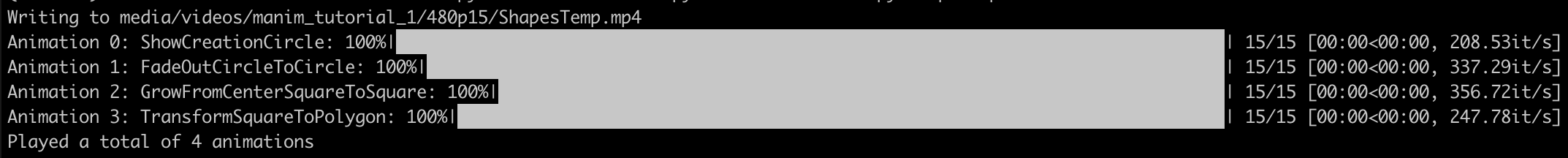
 times the original size and not
  as you might think.
 (see
(see  ) , which manim makes use of. If you’d like to learn more about typesetting with LaTeX I’d recommend the tutorials at
  would be $\alpha$, the angle theta
  would be $\theta$. In manim, however, a double backslash is needed so
  using
using  would be written as $\vec{X}_0$. If the subscript consists of more than a single character you can enclose the subscript in brackets. Thus
  in manim would be $\vec{F}_{net}$.
 ) is the typesetting language that LaTeX is based on so I assume
  . The equation environment doesn’t recognize spaces between words, uses a different font, and spaces the letters differently than normal text.
 .
. R and
R and  } or the set of even numbers which is {
 }), which made list comprehensions click for me. For each item in the list
 is the charge on the point charge,
  is the distance vector between the charge and the observation point, and
  is the magnitude of that vector. The constant out front
 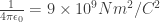 is essentially a conversion factor. For our purposes we will set all constants equal to zero and just look at
 .
. and then the particle is shifted over the distance
  .
.
 . You can also set the distance from the camera to the origin using the keyword argument
  ), which is one of the
  and
and  corresponds to the positive y-axis being ot the right and the positive x-axis being down. This is why
  and
and  corresponds to the normal 2D orientation with the x-axis pointing right and the y-axis pointing up on the screen. If you set
  we flip the screen over.